Nesoil.com - Guide to Interpreting Radar Profiles Note: Most of this article reefers to profiles produced with a
SIR-3 analog radar
The Ground Penetrating Radar (GPR)
records a continuous graphic profile of subsurface interfaces.
The SIR System-3 records images on a gray scale where strong
returning signals (materials with large changes in dielectric
properties), show up on the profile in black and weaker returning
signals show as shades of gray. The SIR-2000 is a digital unit
and profiles are displayed in a variety of colors.
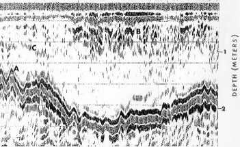
The figure to the right is an example of a graphic profile produced
by the GPR. The horizontal scale represents units of distance
traveled along the transect line. This scale is dependent upon
the speed at which the antenna advances along the transect and
the rate of the paper advance through the graphic recorder (rate
is controlled by the operator). The vertical scale is a time
scale, which represents the amount of time (in nanoseconds) it
takes for the radar pulse to travel through the medium and return
to the antenna. This time scale may be converted into a depth
scale if the velocity of the signal propagation is known (velocity
x time = depth). The dashed vertical lines are event markers
inserted on the profile by the radar operator to indicate known
antenna locations or reference points along the transect lines.
The evenly spaced horizontal lines are scale lines which provide
reference planes for relative depth/time assessments.
Most graphic profiles consist of four basic components: start
of scan image (A), inherent system images (B), surface images (C),
and subsurface images/interfaces (D). All of these components,
with the exception of the start of scan, are generally displayed
in groups of multiple dark bands (positive and negative return
signals) unless limited by high rates of signal attenuation or
the proximity of two or more closely spaced interface signals.
The recorded data represents the total travel time for a GPR
signal to pass from the antenna, through the subsurface to a
reflector, and return to the antenna. A longer time between
transmission and reception of a signal in a given homogeneous
unit generally implies a greater distance to an interface.
Radar Images:
The graphic image produced by the radar can be interpreted by
understanding some basic concepts about the GPR principal of
operation. GPR is a broad band, impulse radar system that has
been specifically designed to penetrate earthen materials.
Relatively high frequency (10 to 1000 MHz), short duration pulses
of energy are transmitted into the ground from a coupled antenna
(mono-static position). Transient electromagnetic waves are
reflected, refracted and diffracted in the subsurface by changes
in electrical conductivity and dielectrical properties. Travel
times and amplitudes of the reflected, refracted and diffracted
waves can be analyzed to give depth, geometry and material type
information.
The continuous profile displayed by the radar unit produces
many types of images, which must be interpreted by the radar
operator. The two main patterns produced by the radar are
interfaces and point objects (figure below). Interfaces are
continuous returns, which typically represents a layer or strata
within the subsurface. Point objects are typically displayed as a
hyperbolic pattern on the profile. Point objects can represent
any type of anomaly in the subsurface from an air filled void to
a buried object.
Establishing depth scales:
As mentioned earlier, the vertical scale of the radar profile
is a time scale which shows the time it takes for the signal to
travel through the subsurface and return to the antenna. This
time scale can be converted to a depth scale if the signal
propagation velocity is known. Propagation velocities can be
either calculated or estimated if ground truthing is not
performed. Calculating the propagation velocity is usually
performed by burying a reflector at a known depth and determining
the velocity using the following formula:
Vm = 2D/t
Where: D = measured depth to reflecting interface. T = elapsed time between transmitted and received pulse (nanoseconds). Vm = effective propagation velocity (feet/nanosecond)
If propagation velocities are known, depths can be estimated
using the following formula:
Depth = Vm(t)/2
Propagation velocities are often estimated using standard
published values for various materials. The following are some
dielectric constants (Er) of various earth materials:
Material
Approximate
Dielectric Constant (Er)
Air
1
Fresh Water
81
Granite
8
Sand, dry (Carver soil)
4.5
Sand, saturated
30
"Average" coarse
loamy soil
12
Ice
4
Using the dielectric constants above, the depth
to an interface may be calculated using the following formula:
D = c(t)/2[(Er)1/2]
Where: D = depth in feet. C = velocity of light (1 foot/nanosecond). T = pulse travel time in nanoseconds. Er = relative dielectric constant of material
Examples of Radar Profiles:
Radar profile of a Hinesburg/Wapanucket
soil, the dark continuous interface is a soil/geologic contact (lithologic
discontinuity) of sandy eolian material underlain by silty
lacustrine sediments.
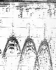
Radar profile showing three buried underground storage tanks,
producing a hyperbolic image.
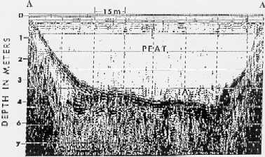
Profile across a peat-filled kettle hole, the dark interface is
the peat/mineral contact (click HERE for
more info).
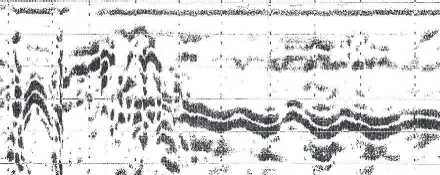
This profile shows an area of high conductivity
between mark 12-17, caused by high nitrate levels in the soil.
The high conductivity causes attenuation of the radar signal. The
dark interface at approximately 1 meter depth is an argillic soil
horizon (Bt horizon).
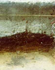
Image
left: Radar profile from and archaeologic site,
the profile shows
a
buried prehistoric Native American corn mound that was
buried by
a meter of eolian sand. Image right:
Soil profile of the excavated
corn mound (dark Apb horizon overlain by quartz sand).